Dimensionality Reduction
If anything is too big to fit in somewhere, what we all do is find ways to some how accomodate it as much as possible. Maybe sugar in a storage box, grocery in shopping bags or even free food. We either split them in different boxes or stuff them in a single container. Maximizing yield.
A way for computers to work with huge files is different file formats. Which compresses the file size while also maintaining the content within.
Similary, when dealing with large datasets one needs to accomodate all the data points. thousands, even millions to get the maximum value of it. It can be to train a model on 10k datapoints to get an accurate prediction or genomic data that contains hundreds of different genes and cell types to study the association. While working with large datapoints, special computer algorithms help in reduction of these datapoint in space hence - “dimension reduction”.
What are these dimensions and why do we need to reduce them?
There are several dimentionality algorithms that can help in this -
- PCA (find the noob version here)
- t SNE
- UMAP
Dimensions are defined as “space” in which data exists.
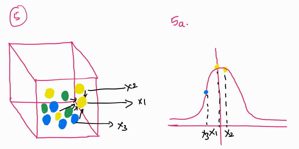
Look at this image. Imagine a box of balls, these balls are occupying a certain space (image 1).
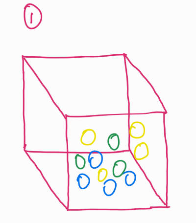
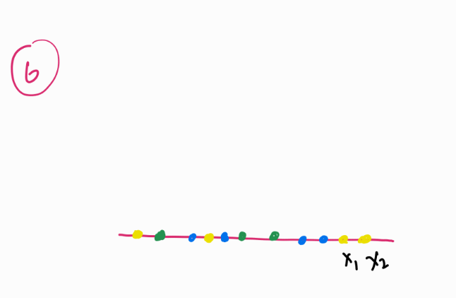
If you plot the location of these balls in 2D, they seem like they are in a single plane (image 2).
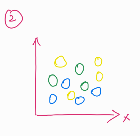
But, for a computer (ML model) to process this information and find meaning in this, these balls present in different dimensions should be reduced to their differences and similarities.
For example we can group these balls into their colors (image 3) and plot them on an X-Y plane, or we can even average out the space occupied by these balls and just plot them, the resultant would be single data points for each color in a 2D plane (image 4).
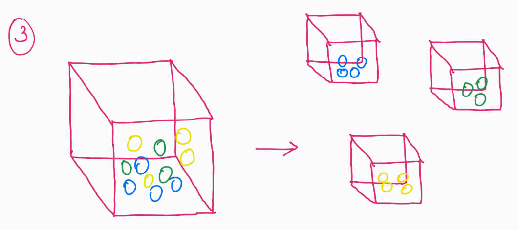
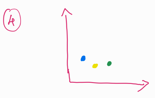
Why is this helpful? Notice that we had 11 balls in image 1, instead of having them as 11 separate data points, we could not reduce it down to just 3. While also keeping its information. In this case, color of the balls.
1. Principle Component Analysis
In PCA, the above examples apply, but instead of just looking at colors,(or other similarities) it is a more mathematical approach of finding similarities or differences in the data point. The common term used is variance. The axes in this is termed as principle components (PCs) and the data points are plotted across these PCs. Now why are these axes given special names you may wonder. For that, watch this quick video on eigenvalues and eigenvectors.
2. t-Distributed Stochastic Neighbor Embedding
The idea of this is similar, mapping high dimensional data to lower dimension still holding important information about the data points. It does so by maintaining the similarities and differences of its neighboring data points.
In t-SNE, the similaritiy between data points is created by taking a gaussian distribution of the other points around it. The probability distribution is calculated for each of the data point in space. Look at Image 5: For the yellow ball (x_1), distances to other points are modeled using a Gaussian distribution centered at x_1. The probability of another point x_2 being close to x_1 is computed as P(2|1) , meaning how likely x_2 is to be a neighbor of x_1. But, this probability is not necessarily symmetric— $P(2|1) \neq P(1|2)$ . To correct this, t-SNE symmetrizes the probabilities by computing:
$P_{12} = \frac{P(2|1) + P(1|2)}{2}$
This captures the pairwise similarity between points in the original high-dimensional space.
In the lower-dimensional space (Image 6), t-SNE tries to replicate these probabilities, but instead of using a Gaussian distribution, it employs a Student’s t-distribution. This choice prevents points from collapsing into a tight cluster and allows better separation of groups. If this does the job similar to PCA then what does t-SNE offer differently?t-SNE works with non-linear data as offers a visually better understanding to spread of data.
3. Uniform Manifold Approximation and Projection
Instead of just looking at distances like PCA or Gaussian probability distributions like t-SNE, UMAP builds a “neighborhood graph”.
For each ball (x_1), UMAP looks at its nearest neighbors (the closest balls around it) and assigns a probability of connection. Unlike t-SNE, which treats all points equally, UMAP allows farther points to have a weaker connection instead of forcing probability distributions on all pairs.
In lower dimensions, UMAP tries to preserve the structure of the graph by keeping close neighbors close together while allowing farther points to spread apart. Instead of using t-distributions (like t-SNE), UMAP optimizes the graph structure using a mathematical cost function.

